Lamont ML Catalog
Contents
Lamont ML Catalog#
This pipeline is developed by the Lamont Group (Wang & Waldhauser). Please explore the overall workflow presented in these slides.
This notebook is part of the SCOPED container for machine learning based earthquake catalog construction. The SCOPED Container page is at https://github.com/SeisSCOPED/ml_catalog
Follow the instructions to pull and run the tutorial container:
To run it on your local machine:#
Install docker from https://docs.docker.com/get-docker/
For Mac: https://docs.docker.com/desktop/install/mac-install/
For Linux: https://docs.docker.com/desktop/install/linux-install/
For Windows: https://docs.docker.com/desktop/install/windows-install/
To run it on AWS cloud (SCOPED workshop users):#
Follow instructions on https://seisscoped.org/HPS-book/chapters/cloud/AWS_101.html to log in to AWS and launching your instance.
When launching your instance (at Step 2), in the Application and OS Images (Amazon Machine Image) block, choose *Architecture as 64-bit (Arm).
Use ‘option 1’ to install docker on your instance. And then pull container image with the command lines below.
Pulling container image#
Use the following commands to pull the container from the GitHub Container Registry (GHCR):
docker pull ghcr.io/seisscoped/ml_catalog:latest

docker run -p 8888:8888 ghcr.io/seisscoped/ml_catalog:latest
For SCOPED workshop users, use:#
sudo docker pull ghcr.io/seisscoped/ml_catalog:latest

sudo docker run -p 8888:8888 ghcr.io/seisscoped/ml_catalog:latest
Run tutorial Jupyter Notebook#
The container will start JupyterLab with a link to open it in a web browser, something like:
To access the notebook, open this file in a browser:
        file:///root/.local/share/jupyter/runtime/nbserver-1-open.html
Or copy and paste one of these URLs:
        http://35e1877ea874:8888/?token=1cfd3a35f9d58cfd52807494ab36dd7166140bb856dbfbb7
or http://127.0.0.1:8888/?token=1cfd3a35f9d58cfd52807494ab36dd7166140bb856dbfbb7
Copy and paste one of the URLs to open it in a browser. Then run the tutorial notebook MLworkflow.ipynb
For SCOPED workshop users,#
Find the Public IPv4 DNS of your AWS instance, replace the IP address in the link with this Public IPv4 DNS and open it in your web browser.
This will open a JupyterLab of the tutorial. Then run the notebook “MLworkflow.ipynb” for machine learning catalog construction workflow.
SCOPED tutorial for ML catalog construction#
This is a Jupyther Notebook of SCOPED tutorial for machine learning catalog construction workflow.
The notebook includes code and examples to download continuous data, detect and pick phases with PhaseNet, assoicate the phases with GaMMA, locate them with HypoInverse, and relocate the events with HypoDD.
Links to the packages/functions:#
Data downloaded with ObsPy Mass Downloader fuction (https://docs.obspy.org/packages/obspy.clients.fdsn.html)
PhaseNet for phase picking (https://github.com/AI4EPS/PhaseNet)
GaMMA for picks association (https://github.com/AI4EPS/GaMMA)
HypoInverse for single event location (https://www.usgs.gov/software/hypoinverse-earthquake-location)
HypoDD for double difference relocation (https://github.com/fwaldhauser/HypoDD)
References:#
Moritz Beyreuther, Robert Barsch, Lion Krischer, Tobias Megies, Yannik Behr and Joachim Wassermann (2010), ObsPy: A Python Toolbox for Seismology, SRL, 81(3), 530-533, doi:10.1785/gssrl.81.3.530.
Zhu, Weiqiang, and Gregory C. Beroza. “PhaseNet: A Deep-Neural-Network-Based Seismic Arrival Time Picking Method.” arXiv preprint arXiv:1803.03211 (2018).
Zhu, Weiqiang et al. “Earthquake Phase Association using a Bayesian Gaussian Mixture Model.” (2021)
Klein, Fred W. User’s guide to HYPOINVERSE-2000, a Fortran program to solve for earthquake locations and magnitudes. No. 2002-171. US Geological Survey, 2002.
Waldhauser, Felix, and William L. Ellsworth, A double-difference earthquake location algorithm: Method and application to the northern Hayward fault, California, Bull. Seism. Soc. Am. 90, 1353-1368, 2000.
ML catalog tutorial: Amatrice, Italy October 2016#
Tutorial Steps:
Download data
Phasenet detection & phase picking
GaMMA Association
HypoInverse location
HypoDD double difference relocation
You might need to change parameters in highlighted lines base on your dataset.
Download data#
Download continous data from IRIS and INGV. Here we download one-day data for test run.
Data downloaded with ObsPy Mass Downloader fuction. See more information at https://docs.obspy.org/packages/obspy.clients.fdsn.html
Data download parameters:
Define study region: latitude, longitude, maxradius
Time range: starttime, endtime
Station information: network, channel_priorities
import obspy
from obspy.clients.fdsn import Client
from obspy import UTCDateTime
from obspy.clients.fdsn.mass_downloader import RectangularDomain, \
    Restrictions, MassDownloader, CircularDomain
from pathlib import Path

domain = CircularDomain(latitude=42.75, longitude=13.25,
                                minradius=0.0, maxradius=1)

wfBaseDir='./waveforms'
Path(wfBaseDir).mkdir(parents=True, exist_ok=True)

restrictions = Restrictions(
    starttime = obspy.UTCDateTime(2016, 10,18,0,0,0),
    endtime   = obspy.UTCDateTime(2016, 10,18,0,10,0),
    chunklength_in_sec=86400,
    network="YR,IV",
    channel_priorities=["[HE][HN]?"],
    reject_channels_with_gaps=False,
    minimum_length=0.0,
    minimum_interstation_distance_in_m=100.0)

mdl = MassDownloader(providers=["IRIS", "INGV"])
mdl.download(domain, restrictions,
             mseed_storage=wfBaseDir+"/{network}/{station}/"
                         "{channel}.{location}.{starttime}.{endtime}.mseed",
             stationxml_storage="stations")
[2024-04-28 00:50:18,097] - obspy.clients.fdsn.mass_downloader - INFO: Initializing FDSN client(s) for IRIS, INGV.
[2024-04-28 00:50:18,761] - obspy.clients.fdsn.mass_downloader - INFO: Successfully initialized 2 client(s): IRIS, INGV.
[2024-04-28 00:50:18,764] - obspy.clients.fdsn.mass_downloader - INFO: Total acquired or preexisting stations: 0
[2024-04-28 00:50:18,765] - obspy.clients.fdsn.mass_downloader - INFO: Client 'IRIS' - Requesting reliable availability.
[2024-04-28 00:50:19,471] - obspy.clients.fdsn.mass_downloader - INFO: Client 'IRIS' - Successfully requested availability (0.71 seconds)
[2024-04-28 00:50:19,474] - obspy.clients.fdsn.mass_downloader - INFO: Client 'IRIS' - Found 24 stations (72 channels).
[2024-04-28 00:50:19,481] - obspy.clients.fdsn.mass_downloader - INFO: Client 'IRIS' - Will attempt to download data from 24 stations.
[2024-04-28 00:50:19,484] - obspy.clients.fdsn.mass_downloader - INFO: Client 'IRIS' - Status for 72 time intervals/channels before downloading: EXISTS
[2024-04-28 00:50:19,575] - obspy.clients.fdsn.mass_downloader - INFO: Client 'IRIS' - No station information to download.
[2024-04-28 00:50:19,575] - obspy.clients.fdsn.mass_downloader - INFO: Total acquired or preexisting stations: 24
[2024-04-28 00:50:19,576] - obspy.clients.fdsn.mass_downloader - INFO: Client 'INGV' - Requesting unreliable availability.
[2024-04-28 00:50:22,677] - obspy.clients.fdsn.mass_downloader - INFO: Client 'INGV' - Successfully requested availability (3.10 seconds)
[2024-04-28 00:50:22,709] - obspy.clients.fdsn.mass_downloader - INFO: Client 'INGV' - Found 80 stations (318 channels).
[2024-04-28 00:50:22,710] - obspy.clients.fdsn.mass_downloader - INFO: Client 'INGV' - Will attempt to download data from 80 stations.
[2024-04-28 00:50:22,721] - obspy.clients.fdsn.mass_downloader - INFO: Client 'INGV' - Status for 273 time intervals/channels before downloading: EXISTS
[2024-04-28 00:50:22,722] - obspy.clients.fdsn.mass_downloader - INFO: Client 'INGV' - Status for 45 time intervals/channels before downloading: NEEDS_DOWNLOADING
[2024-04-28 00:50:24,863] - obspy.clients.fdsn.mass_downloader - INFO: Client 'INGV' - No data available for request.
HTTP Status code: 204
[2024-04-28 00:50:24,866] - obspy.clients.fdsn.mass_downloader - INFO: Client 'INGV' - Launching basic QC checks...
[2024-04-28 00:50:24,870] - obspy.clients.fdsn.mass_downloader - INFO: Client 'INGV' - Downloaded 0.0 MB [0.00 KB/sec] of data, 0.0 MB of which were discarded afterwards.
[2024-04-28 00:50:24,872] - obspy.clients.fdsn.mass_downloader - INFO: Client 'INGV' - Status for 45 time intervals/channels after downloading: DOWNLOAD_FAILED
[2024-04-28 00:50:24,874] - obspy.clients.fdsn.mass_downloader - INFO: Client 'INGV' - Status for 273 time intervals/channels after downloading: EXISTS
[2024-04-28 00:50:24,964] - obspy.clients.fdsn.mass_downloader - INFO: Client 'INGV' - No station information to download.
[2024-04-28 00:50:24,978] - obspy.clients.fdsn.mass_downloader - INFO: ============================== Final report
[2024-04-28 00:50:24,980] - obspy.clients.fdsn.mass_downloader - INFO: 345 MiniSEED files [34.7 MB] already existed.
[2024-04-28 00:50:24,981] - obspy.clients.fdsn.mass_downloader - INFO: 92 StationXML files [8.9 MB] already existed.
[2024-04-28 00:50:24,982] - obspy.clients.fdsn.mass_downloader - INFO: Client 'IRIS' - Acquired 0 MiniSEED files [0.0 MB].
[2024-04-28 00:50:24,983] - obspy.clients.fdsn.mass_downloader - INFO: Client 'IRIS' - Acquired 0 StationXML files [0.0 MB].
[2024-04-28 00:50:24,983] - obspy.clients.fdsn.mass_downloader - INFO: Client 'INGV' - Acquired 0 MiniSEED files [0.0 MB].
[2024-04-28 00:50:24,984] - obspy.clients.fdsn.mass_downloader - INFO: Client 'INGV' - Acquired 0 StationXML files [0.0 MB].
[2024-04-28 00:50:24,984] - obspy.clients.fdsn.mass_downloader - INFO: Downloaded 0.0 MB in total.
{'IRIS': <obspy.clients.fdsn.mass_downloader.download_helpers.ClientDownloadHelper at 0xffff845b25f0>,
 'INGV': <obspy.clients.fdsn.mass_downloader.download_helpers.ClientDownloadHelper at 0xffff38668ca0>}
Prepare PhaseNet input files and running PhaseNet for phase picking#
PhaseNet model from https://github.com/AI4EPS/PhaseNet
Reference:#
Zhu, Weiqiang, and Gregory C. Beroza. “PhaseNet: A Deep-Neural-Network-Based Seismic Arrival Time Picking Method.” arXiv preprint arXiv:1803.03211 (2018).
Write input waveform file path from the downloaded miniseed waveforms:#
write input files required by PhaseNet: use the miniseed data we just downloaded
import glob
import numpy as np

PhasenetResultDir='./results_phasenet'
Path(PhasenetResultDir).mkdir(parents=True, exist_ok=True)
mseed_path=wfBaseDir+'/*/*/*.mseed'
filenames = glob.glob(mseed_path)

filenames=['./'+file.split('/')[2]+'/'+file.split('/')[3]+'/*.*.'+(file.split('/')[-1]).split('.')[2]+'.*.mseed' for file in filenames]
filenames=np.unique(filenames)
print('number of stations',len(filenames))
filenames=np.insert(filenames, 0, 'fname')

np.savetxt(PhasenetResultDir+'/mseed.csv', filenames, fmt='%s')
number of stations 92
Write station file from the .xml files:#
generate input station file with the .xml files we just downloaded
from obspy import read_inventory
from collections import defaultdict
import pandas as pd
inv = read_inventory("./stations/*.xml")

station_locs = defaultdict(dict)
stations=inv
for network in stations:
    for station in network:
        for chn in station:
            sid = f"{network.code}.{station.code}.{chn.location_code}.{chn.code[:-1]}"
            if sid in station_locs:
                station_locs[sid]["component"] += f",{chn.code[-1]}"
                station_locs[sid]["response"] += f",{chn.response.instrument_sensitivity.value:.2f}"
            else:
                component = f"{chn.code[-1]}"
                response = f"{chn.response.instrument_sensitivity.value:.2f}"
                dtype = chn.response.instrument_sensitivity.input_units.lower()
                tmp_dict = {}
                tmp_dict["longitude"], tmp_dict["latitude"], tmp_dict["elevation(m)"] = (
                    chn.longitude,
                    chn.latitude,
                    chn.elevation,
                )
                tmp_dict["component"], tmp_dict["response"], tmp_dict["unit"] = component, response, dtype
                station_locs[sid] = tmp_dict
            if station_locs[sid]["component"]=='Z':
                station_locs[sid]["response"]= f"0,0,"+station_locs[sid]["response"]
            elif station_locs[sid]["component"]=='N,Z':
                station_locs[sid]["response"]= f"0,"+station_locs[sid]["response"]
station_locs = pd.DataFrame.from_dict(station_locs, orient='index')
station_locs["id"] = station_locs.index
station_locs = station_locs.rename_axis('station').reset_index()
station_locs.to_csv("./stations.csv",sep='\t')
station_locs
| station | longitude | latitude | elevation(m) | component | response | unit | id | |
|---|---|---|---|---|---|---|---|---|
| 0 | IV.AOI..HH | 13.60200 | 43.550170 | 530.0 | E,N,Z | 1179650000.00,1179650000.00,1179650000.00 | m/s | IV.AOI..HH |
| 1 | IV.ARRO..EH | 12.76567 | 42.579170 | 253.0 | E,N,Z | 503316000.00,503316000.00,503316000.00 | m/s | IV.ARRO..EH |
| 2 | IV.ARVD..HH | 12.94153 | 43.498070 | 461.0 | E,N,Z | 1179650000.00,1179650000.00,1179650000.00 | m/s | IV.ARVD..HH |
| 3 | IV.ASSB..HH | 12.65870 | 43.042600 | 734.0 | E,N,Z | 8823530000.00,8823530000.00,8823530000.00 | m/s | IV.ASSB..HH |
| 4 | IV.ATBU..EH | 12.54828 | 43.475710 | 1000.0 | E,N,Z | 503316000.00,503316000.00,503316000.00 | m/s | IV.ATBU..EH |
| ... | ... | ... | ... | ... | ... | ... | ... | ... |
| 110 | YR.ED21..HH | 13.27227 | 43.030071 | 720.0 | E,N,Z | 2463140000.00,2456910000.00,2455960000.00 | m/s | YR.ED21..HH |
| 111 | YR.ED22..HH | 13.32520 | 43.006748 | 620.0 | E,N,Z | 2417850000.00,2419350000.00,2423940000.00 | m/s | YR.ED22..HH |
| 112 | YR.ED23..HH | 13.28710 | 42.743191 | 1045.0 | E,N,Z | 2318760000.00,2340510000.00,2317430000.00 | m/s | YR.ED23..HH |
| 113 | YR.ED24..HH | 13.19232 | 42.655640 | 1104.0 | E,N,Z | 2488010000.00,2543750000.00,2506750000.00 | m/s | YR.ED24..HH |
| 114 | YR.ED25..HH | 13.35188 | 42.598770 | 1353.0 | E,N,Z | 2452670000.00,2452210000.00,2448100000.00 | m/s | YR.ED25..HH |
115 rows × 8 columns
Run PhaseNet#
Phase picking on continous data. Output phase picks for given station and waveform files.
!python ./phasenet/predict.py --model=./phasenet/model/190703-214543 --data_list=./results_phasenet/mseed.csv --data_dir=./waveforms --format=mseed_array --amplitude --result_dir=./results_phasenet/result/ --stations=./stations.csv
     Unnamed: 0      station  ...  unit           id
0             0   IV.AOI..HH  ...   m/s   IV.AOI..HH
1             1  IV.ARRO..EH  ...   m/s  IV.ARRO..EH
2             2  IV.ARVD..HH  ...   m/s  IV.ARVD..HH
3             3  IV.ASSB..HH  ...   m/s  IV.ASSB..HH
4             4  IV.ATBU..EH  ...   m/s  IV.ATBU..EH
..          ...          ...  ...   ...          ...
110         110  YR.ED21..HH  ...   m/s  YR.ED21..HH
111         111  YR.ED22..HH  ...   m/s  YR.ED22..HH
112         112  YR.ED23..HH  ...   m/s  YR.ED23..HH
113         113  YR.ED24..HH  ...   m/s  YR.ED24..HH
114         114  YR.ED25..HH  ...   m/s  YR.ED25..HH

[115 rows x 9 columns]
2024-04-28 00:50:28,578 Pred log: ./results_phasenet/result/
2024-04-28 00:50:28,578 Dataset size: 92
2024-04-28 00:50:28,630 Model: depths 5, filters 8, filter size 7x1, pool size: 4x1, dilation rate: 1x1
/app/phasenet/model.py:158: UserWarning: `tf.layers.conv2d` is deprecated and will be removed in a future version. Please Use `tf.keras.layers.Conv2D` instead.
  net = tf.compat.v1.layers.conv2d(net,
/app/phasenet/model.py:167: UserWarning: `tf.layers.batch_normalization` is deprecated and will be removed in a future version. Please use `tf.keras.layers.BatchNormalization` instead. In particular, `tf.control_dependencies(tf.GraphKeys.UPDATE_OPS)` should not be used (consult the `tf.keras.layers.BatchNormalization` documentation).
  net = tf.compat.v1.layers.batch_normalization(net,
/app/phasenet/model.py:173: UserWarning: `tf.layers.dropout` is deprecated and will be removed in a future version. Please use `tf.keras.layers.Dropout` instead.
  net = tf.compat.v1.layers.dropout(net,
/app/phasenet/model.py:183: UserWarning: `tf.layers.conv2d` is deprecated and will be removed in a future version. Please Use `tf.keras.layers.Conv2D` instead.
  net = tf.compat.v1.layers.conv2d(net,
/app/phasenet/model.py:193: UserWarning: `tf.layers.batch_normalization` is deprecated and will be removed in a future version. Please use `tf.keras.layers.BatchNormalization` instead. In particular, `tf.control_dependencies(tf.GraphKeys.UPDATE_OPS)` should not be used (consult the `tf.keras.layers.BatchNormalization` documentation).
  net = tf.compat.v1.layers.batch_normalization(net,
/app/phasenet/model.py:198: UserWarning: `tf.layers.dropout` is deprecated and will be removed in a future version. Please use `tf.keras.layers.Dropout` instead.
  net = tf.compat.v1.layers.dropout(net,
/app/phasenet/model.py:206: UserWarning: `tf.layers.conv2d` is deprecated and will be removed in a future version. Please Use `tf.keras.layers.Conv2D` instead.
  net = tf.compat.v1.layers.conv2d(net,
/app/phasenet/model.py:217: UserWarning: `tf.layers.batch_normalization` is deprecated and will be removed in a future version. Please use `tf.keras.layers.BatchNormalization` instead. In particular, `tf.control_dependencies(tf.GraphKeys.UPDATE_OPS)` should not be used (consult the `tf.keras.layers.BatchNormalization` documentation).
  net = tf.compat.v1.layers.batch_normalization(net,
/app/phasenet/model.py:222: UserWarning: `tf.layers.dropout` is deprecated and will be removed in a future version. Please use `tf.keras.layers.Dropout` instead.
  net = tf.compat.v1.layers.dropout(net,
/app/phasenet/model.py:232: UserWarning: `tf.layers.conv2d_transpose` is deprecated and will be removed in a future version. Please Use `tf.keras.layers.Conv2DTranspose` instead.
  net = tf.compat.v1.layers.conv2d_transpose(net,
/app/phasenet/model.py:242: UserWarning: `tf.layers.batch_normalization` is deprecated and will be removed in a future version. Please use `tf.keras.layers.BatchNormalization` instead. In particular, `tf.control_dependencies(tf.GraphKeys.UPDATE_OPS)` should not be used (consult the `tf.keras.layers.BatchNormalization` documentation).
  net = tf.compat.v1.layers.batch_normalization(net,
/app/phasenet/model.py:247: UserWarning: `tf.layers.dropout` is deprecated and will be removed in a future version. Please use `tf.keras.layers.Dropout` instead.
  net = tf.compat.v1.layers.dropout(net,
/app/phasenet/model.py:257: UserWarning: `tf.layers.conv2d` is deprecated and will be removed in a future version. Please Use `tf.keras.layers.Conv2D` instead.
  net = tf.compat.v1.layers.conv2d(net,
/app/phasenet/model.py:267: UserWarning: `tf.layers.batch_normalization` is deprecated and will be removed in a future version. Please use `tf.keras.layers.BatchNormalization` instead. In particular, `tf.control_dependencies(tf.GraphKeys.UPDATE_OPS)` should not be used (consult the `tf.keras.layers.BatchNormalization` documentation).
  net = tf.compat.v1.layers.batch_normalization(net,
/app/phasenet/model.py:272: UserWarning: `tf.layers.dropout` is deprecated and will be removed in a future version. Please use `tf.keras.layers.Dropout` instead.
  net = tf.compat.v1.layers.dropout(net,
/app/phasenet/model.py:280: UserWarning: `tf.layers.conv2d` is deprecated and will be removed in a future version. Please Use `tf.keras.layers.Conv2D` instead.
  net = tf.compat.v1.layers.conv2d(net,
2024-04-28 00:50:29.430408: I tensorflow/compiler/mlir/mlir_graph_optimization_pass.cc:388] MLIR V1 optimization pass is not enabled
2024-04-28 00:50:29,540 restoring model ./phasenet/model/190703-214543/model_95.ckpt
Pred:   3%|█▏                                    | 3/92 [00:00<00:20,  4.38it/s]2024-04-28 00:50:30,357 Resampling IV.ATCC..HNE from 200.0 to 100 Hz
2024-04-28 00:50:30,363 Resampling IV.ATCC..HNN from 200.0 to 100 Hz
2024-04-28 00:50:30,366 Resampling IV.ATCC..HNZ from 200.0 to 100 Hz
Pred:   4%|█▋                                    | 4/92 [00:00<00:18,  4.83it/s]2024-04-28 00:50:30,531 Resampling IV.ATFO..HNE from 200.0 to 100 Hz
2024-04-28 00:50:30,534 Resampling IV.ATFO..HNN from 200.0 to 100 Hz
2024-04-28 00:50:30,536 Resampling IV.ATFO..HNZ from 200.0 to 100 Hz
Pred:   5%|██                                    | 5/92 [00:01<00:16,  5.12it/s]2024-04-28 00:50:30,705 Resampling IV.ATLO..HNE from 200.0 to 100 Hz
2024-04-28 00:50:30,708 Resampling IV.ATLO..HNN from 200.0 to 100 Hz
2024-04-28 00:50:30,710 Resampling IV.ATLO..HNZ from 200.0 to 100 Hz
Pred:   8%|██▉                                   | 7/92 [00:01<00:23,  3.63it/s]2024-04-28 00:50:31,385 Resampling IV.ATPC..HNE from 200.0 to 100 Hz
2024-04-28 00:50:31,387 Resampling IV.ATPC..HNN from 200.0 to 100 Hz
2024-04-28 00:50:31,390 Resampling IV.ATPC..HNZ from 200.0 to 100 Hz
Pred:  11%|████                                 | 10/92 [00:02<00:23,  3.54it/s]2024-04-28 00:50:32,235 Resampling IV.ATTE..HNE from 200.0 to 100 Hz
2024-04-28 00:50:32,238 Resampling IV.ATTE..HNN from 200.0 to 100 Hz
2024-04-28 00:50:32,240 Resampling IV.ATTE..HNZ from 200.0 to 100 Hz
Pred:  13%|████▊                                | 12/92 [00:02<00:18,  4.42it/s]2024-04-28 00:50:32,585 Resampling IV.ATVO..HNE from 200.0 to 100 Hz
2024-04-28 00:50:32,587 Resampling IV.ATVO..HNN from 200.0 to 100 Hz
2024-04-28 00:50:32,590 Resampling IV.ATVO..HNZ from 200.0 to 100 Hz
Pred:  14%|█████▏                               | 13/92 [00:03<00:20,  3.84it/s]2024-04-28 00:50:32,923 Resampling IV.CADA..HNE from 200.0 to 100 Hz
2024-04-28 00:50:32,925 Resampling IV.CADA..HNN from 200.0 to 100 Hz
2024-04-28 00:50:32,928 Resampling IV.CADA..HNZ from 200.0 to 100 Hz
Pred:  20%|███████▏                             | 18/92 [00:04<00:15,  4.88it/s]2024-04-28 00:50:33,953 Resampling IV.CIMA..HNE from 200.0 to 100 Hz
2024-04-28 00:50:33,955 Resampling IV.CIMA..HNN from 200.0 to 100 Hz
2024-04-28 00:50:33,958 Resampling IV.CIMA..HNZ from 200.0 to 100 Hz
Pred:  22%|████████                             | 20/92 [00:04<00:13,  5.28it/s]2024-04-28 00:50:34,303 Resampling IV.COR1..HNE from 200.0 to 100 Hz
2024-04-28 00:50:34,304 Resampling IV.COR1..HNE from 200.0 to 100 Hz
2024-04-28 00:50:34,304 Resampling IV.COR1..HNN from 200.0 to 100 Hz
2024-04-28 00:50:34,304 Resampling IV.COR1..HNN from 200.0 to 100 Hz
2024-04-28 00:50:34,304 Resampling IV.COR1..HNZ from 200.0 to 100 Hz
2024-04-28 00:50:34,305 Resampling IV.COR1..HNZ from 200.0 to 100 Hz
Pred:  25%|█████████▎                           | 23/92 [00:05<00:15,  4.37it/s]2024-04-28 00:50:34,990 Resampling IV.FEMA..HNE from 200.0 to 100 Hz
2024-04-28 00:50:34,993 Resampling IV.FEMA..HNN from 200.0 to 100 Hz
2024-04-28 00:50:34,995 Resampling IV.FEMA..HNZ from 200.0 to 100 Hz
Pred:  27%|██████████                           | 25/92 [00:05<00:13,  5.01it/s]2024-04-28 00:50:35,333 Resampling IV.FIU1..HNE from 200.0 to 100 Hz
2024-04-28 00:50:35,336 Resampling IV.FIU1..HNN from 200.0 to 100 Hz
2024-04-28 00:50:35,338 Resampling IV.FIU1..HNZ from 200.0 to 100 Hz
Pred:  28%|██████████▍                          | 26/92 [00:05<00:12,  5.24it/s]2024-04-28 00:50:35,505 Resampling IV.FOSV..HNE from 200.0 to 100 Hz
2024-04-28 00:50:35,508 Resampling IV.FOSV..HNN from 200.0 to 100 Hz
2024-04-28 00:50:35,510 Resampling IV.FOSV..HNZ from 200.0 to 100 Hz
Pred:  30%|███████████▎                         | 28/92 [00:06<00:13,  4.58it/s]2024-04-28 00:50:36,024 Resampling IV.GAG1..HNE from 200.0 to 100 Hz
2024-04-28 00:50:36,026 Resampling IV.GAG1..HNN from 200.0 to 100 Hz
2024-04-28 00:50:36,029 Resampling IV.GAG1..HNZ from 200.0 to 100 Hz
Pred:  34%|████████████▍                        | 31/92 [00:07<00:12,  4.71it/s]2024-04-28 00:50:36,710 Resampling IV.GUMA..HNE from 200.0 to 100 Hz
2024-04-28 00:50:36,712 Resampling IV.GUMA..HNN from 200.0 to 100 Hz
2024-04-28 00:50:36,715 Resampling IV.GUMA..HNZ from 200.0 to 100 Hz
Pred:  35%|████████████▊                        | 32/92 [00:07<00:12,  4.99it/s]2024-04-28 00:50:36,882 Resampling IV.INTR..HNE from 200.0 to 100 Hz
2024-04-28 00:50:36,885 Resampling IV.INTR..HNN from 200.0 to 100 Hz
2024-04-28 00:50:36,887 Resampling IV.INTR..HNZ from 200.0 to 100 Hz
Pred:  39%|██████████████▍                      | 36/92 [00:08<00:13,  4.22it/s]2024-04-28 00:50:37,897 Resampling IV.MDAR..HNE from 200.0 to 100 Hz
2024-04-28 00:50:37,900 Resampling IV.MDAR..HNN from 200.0 to 100 Hz
2024-04-28 00:50:37,902 Resampling IV.MDAR..HNZ from 200.0 to 100 Hz
Pred:  41%|███████████████▎                     | 38/92 [00:08<00:11,  4.90it/s]2024-04-28 00:50:38,244 Resampling IV.MMO1..HNE from 200.0 to 100 Hz
2024-04-28 00:50:38,244 Resampling IV.MMO1..HNE from 200.0 to 100 Hz
2024-04-28 00:50:38,246 Resampling IV.MMO1..HNE from 200.0 to 100 Hz
2024-04-28 00:50:38,247 Resampling IV.MMO1..HNN from 200.0 to 100 Hz
2024-04-28 00:50:38,247 Resampling IV.MMO1..HNN from 200.0 to 100 Hz
2024-04-28 00:50:38,249 Resampling IV.MMO1..HNN from 200.0 to 100 Hz
2024-04-28 00:50:38,250 Resampling IV.MMO1..HNZ from 200.0 to 100 Hz
2024-04-28 00:50:38,250 Resampling IV.MMO1..HNZ from 200.0 to 100 Hz
2024-04-28 00:50:38,252 Resampling IV.MMO1..HNZ from 200.0 to 100 Hz
Pred:  42%|███████████████▋                     | 39/92 [00:08<00:10,  5.15it/s]2024-04-28 00:50:38,413 Resampling IV.MMUR..HNE from 200.0 to 100 Hz
2024-04-28 00:50:38,415 Resampling IV.MMUR..HNN from 200.0 to 100 Hz
2024-04-28 00:50:38,417 Resampling IV.MMUR..HNZ from 200.0 to 100 Hz
Pred:  43%|████████████████                     | 40/92 [00:09<00:12,  4.19it/s]2024-04-28 00:50:38,756 Resampling IV.MNTP..HNE from 200.0 to 100 Hz
2024-04-28 00:50:38,759 Resampling IV.MNTP..HNN from 200.0 to 100 Hz
2024-04-28 00:50:38,761 Resampling IV.MNTP..HNZ from 200.0 to 100 Hz
Pred:  45%|████████████████▍                    | 41/92 [00:09<00:13,  3.72it/s]2024-04-28 00:50:39,098 Resampling IV.MPAG..HNE from 200.0 to 100 Hz
2024-04-28 00:50:39,101 Resampling IV.MPAG..HNE from 200.0 to 100 Hz
2024-04-28 00:50:39,101 Resampling IV.MPAG..HNN from 200.0 to 100 Hz
2024-04-28 00:50:39,103 Resampling IV.MPAG..HNN from 200.0 to 100 Hz
2024-04-28 00:50:39,103 Resampling IV.MPAG..HNZ from 200.0 to 100 Hz
2024-04-28 00:50:39,106 Resampling IV.MPAG..HNZ from 200.0 to 100 Hz
Pred:  47%|█████████████████▎                   | 43/92 [00:09<00:10,  4.56it/s]2024-04-28 00:50:39,438 Resampling IV.MTL1..HNE from 200.0 to 100 Hz
2024-04-28 00:50:39,441 Resampling IV.MTL1..HNN from 200.0 to 100 Hz
2024-04-28 00:50:39,443 Resampling IV.MTL1..HNZ from 200.0 to 100 Hz
Pred:  48%|█████████████████▋                   | 44/92 [00:10<00:12,  3.92it/s]2024-04-28 00:50:39,781 Resampling IV.MURB..HNE from 200.0 to 100 Hz
2024-04-28 00:50:39,783 Resampling IV.MURB..HNN from 200.0 to 100 Hz
2024-04-28 00:50:39,786 Resampling IV.MURB..HNZ from 200.0 to 100 Hz
Pred:  50%|██████████████████▌                  | 46/92 [00:10<00:09,  4.70it/s]2024-04-28 00:50:40,123 Resampling IV.NRCA..HNE from 200.0 to 100 Hz
2024-04-28 00:50:40,126 Resampling IV.NRCA..HNN from 200.0 to 100 Hz
2024-04-28 00:50:40,128 Resampling IV.NRCA..HNZ from 200.0 to 100 Hz
Pred:  52%|███████████████████▎                 | 48/92 [00:11<00:10,  4.38it/s]2024-04-28 00:50:40,641 Resampling IV.PCRO..HNE from 200.0 to 100 Hz
2024-04-28 00:50:40,646 Resampling IV.PCRO..HNN from 200.0 to 100 Hz
2024-04-28 00:50:40,650 Resampling IV.PCRO..HNZ from 200.0 to 100 Hz
Pred:  53%|███████████████████▋                 | 49/92 [00:11<00:11,  3.79it/s]2024-04-28 00:50:40,985 Resampling IV.PIEI..HNE from 200.0 to 100 Hz
2024-04-28 00:50:40,987 Resampling IV.PIEI..HNN from 200.0 to 100 Hz
2024-04-28 00:50:40,990 Resampling IV.PIEI..HNZ from 200.0 to 100 Hz
Pred:  54%|████████████████████                 | 50/92 [00:11<00:09,  4.23it/s]2024-04-28 00:50:41,157 Resampling IV.PIO1..HNE from 200.0 to 100 Hz
2024-04-28 00:50:41,160 Resampling IV.PIO1..HNN from 200.0 to 100 Hz
2024-04-28 00:50:41,162 Resampling IV.PIO1..HNZ from 200.0 to 100 Hz
Pred:  55%|████████████████████▌                | 51/92 [00:11<00:08,  4.60it/s]2024-04-28 00:50:41,331 Resampling IV.PP3..HNE from 200.0 to 100 Hz
2024-04-28 00:50:41,334 Resampling IV.PP3..HNN from 200.0 to 100 Hz
2024-04-28 00:50:41,336 Resampling IV.PP3..HNZ from 200.0 to 100 Hz
Pred:  59%|█████████████████████▋               | 54/92 [00:12<00:09,  3.83it/s]2024-04-28 00:50:42,177 Resampling IV.RM33..HNE from 200.0 to 100 Hz
2024-04-28 00:50:42,179 Resampling IV.RM33..HNN from 200.0 to 100 Hz
2024-04-28 00:50:42,182 Resampling IV.RM33..HNZ from 200.0 to 100 Hz
Pred:  60%|██████████████████████               | 55/92 [00:12<00:08,  4.26it/s]2024-04-28 00:50:42,349 Resampling IV.SEF1..HNE from 200.0 to 100 Hz
2024-04-28 00:50:42,349 Resampling IV.SEF1..HNE from 200.0 to 100 Hz
2024-04-28 00:50:42,351 Resampling IV.SEF1..HNN from 200.0 to 100 Hz
2024-04-28 00:50:42,352 Resampling IV.SEF1..HNN from 200.0 to 100 Hz
2024-04-28 00:50:42,352 Resampling IV.SEF1..HNN from 200.0 to 100 Hz
2024-04-28 00:50:42,354 Resampling IV.SEF1..HNZ from 200.0 to 100 Hz
2024-04-28 00:50:42,354 Resampling IV.SEF1..HNZ from 200.0 to 100 Hz
2024-04-28 00:50:42,355 Resampling IV.SEF1..HNZ from 200.0 to 100 Hz
Pred:  61%|██████████████████████▌              | 56/92 [00:12<00:07,  4.64it/s]2024-04-28 00:50:42,522 Resampling IV.SENI..HNE from 200.0 to 100 Hz
2024-04-28 00:50:42,523 Resampling IV.SENI..HNE from 200.0 to 100 Hz
2024-04-28 00:50:42,524 Resampling IV.SENI..HNE from 200.0 to 100 Hz
2024-04-28 00:50:42,525 Resampling IV.SENI..HNE from 200.0 to 100 Hz
2024-04-28 00:50:42,525 Resampling IV.SENI..HNN from 200.0 to 100 Hz
2024-04-28 00:50:42,526 Resampling IV.SENI..HNN from 200.0 to 100 Hz
2024-04-28 00:50:42,527 Resampling IV.SENI..HNN from 200.0 to 100 Hz
2024-04-28 00:50:42,528 Resampling IV.SENI..HNN from 200.0 to 100 Hz
2024-04-28 00:50:42,528 Resampling IV.SENI..HNZ from 200.0 to 100 Hz
2024-04-28 00:50:42,528 Resampling IV.SENI..HNZ from 200.0 to 100 Hz
2024-04-28 00:50:42,530 Resampling IV.SENI..HNZ from 200.0 to 100 Hz
2024-04-28 00:50:42,531 Resampling IV.SENI..HNZ from 200.0 to 100 Hz
Pred:  63%|███████████████████████▎             | 58/92 [00:13<00:07,  4.36it/s]2024-04-28 00:50:43,036 Resampling IV.SNTG..HNE from 200.0 to 100 Hz
2024-04-28 00:50:43,039 Resampling IV.SNTG..HNN from 200.0 to 100 Hz
2024-04-28 00:50:43,041 Resampling IV.SNTG..HNZ from 200.0 to 100 Hz
Pred:  65%|████████████████████████▏            | 60/92 [00:13<00:07,  4.27it/s]2024-04-28 00:50:43,545 Resampling IV.SSM1..HNE from 200.0 to 100 Hz
2024-04-28 00:50:43,545 Resampling IV.SSM1..HNE from 200.0 to 100 Hz
2024-04-28 00:50:43,547 Resampling IV.SSM1..HNN from 200.0 to 100 Hz
2024-04-28 00:50:43,548 Resampling IV.SSM1..HNN from 200.0 to 100 Hz
2024-04-28 00:50:43,550 Resampling IV.SSM1..HNZ from 200.0 to 100 Hz
2024-04-28 00:50:43,550 Resampling IV.SSM1..HNZ from 200.0 to 100 Hz
Pred:  66%|████████████████████████▌            | 61/92 [00:14<00:08,  3.72it/s]2024-04-28 00:50:43,895 Resampling IV.T1299..HNE from 200.0 to 100 Hz
2024-04-28 00:50:43,896 Resampling IV.T1299..HNE from 200.0 to 100 Hz
2024-04-28 00:50:43,897 Resampling IV.T1299..HNN from 200.0 to 100 Hz
2024-04-28 00:50:43,899 Resampling IV.T1299..HNN from 200.0 to 100 Hz
2024-04-28 00:50:43,900 Resampling IV.T1299..HNZ from 200.0 to 100 Hz
2024-04-28 00:50:43,901 Resampling IV.T1299..HNZ from 200.0 to 100 Hz
Pred: 100%|█████████████████████████████████████| 92/92 [00:19<00:00,  4.62it/s]
Done with 1090 P-picks and 1105 S-picks
Run GaMMA#
Associating PhaseNet picks into events with GaMMA (https://github.com/AI4EPS/GaMMA)
Reference:#
Zhu, Weiqiang et al. “Earthquake Phase Association using a Bayesian Gaussian Mixture Model.” (2021)
Set GaMMA parameters:#
Parameters you might want to change based on your dataset:
Define study region: center=(latitude, longitude), horizontal_degree, vertical_degree, z(km)
Time range: starttime, endtime
Station information: network_list, channel_list
Association parameters:
dbscan_eps (for sparse network use a larger number)
min_picks_per_eq (minimum number of associated picks per event)
max_sigma11 (a larger value allows larger pick uncertainty)
GMMAResultDir='./GMMA'
Path(GMMAResultDir).mkdir(parents=True, exist_ok=True)

catalog_csv = GMMAResultDir+"/catalog_gamma.csv"
picks_csv = GMMAResultDir+"/picks_gamma.csv"


region_name = "Italy"
center = (13.2, 42.7)
horizontal_degree = 0.85
vertical_degree = 0.85
starttime = obspy.UTCDateTime("2016-10-18T00")
endtime =   obspy.UTCDateTime("2016-10-19T00")
network_list = ["IV","YR"]
channel_list = "HH*,EH*,HN*,EN*"

config = {}
config["region"] = region_name
config["center"] = center
config["xlim_degree"] = [center[0] - horizontal_degree / 2, center[0] + horizontal_degree / 2]
config["ylim_degree"] = [center[1] - vertical_degree / 2, center[1] + vertical_degree / 2]
config["starttime"] = starttime.datetime.isoformat()
config["endtime"] = endtime.datetime.isoformat()
config["networks"] = network_list
config["channels"] = channel_list
config["degree2km"] = 111
config["degree2km_x"] = 82
config['vel']= {"p":6.2, "s":3.3}


config["dims"] = ['x(km)', 'y(km)', 'z(km)']
config["use_dbscan"] = True
config["use_amplitude"] = True
config["x(km)"] = (np.array(config["xlim_degree"])-np.array(config["center"][0]))*config["degree2km_x"]
config["y(km)"] = (np.array(config["ylim_degree"])-np.array(config["center"][1]))*config["degree2km"]
config["z(km)"] = (0, 20)

# DBSCAN
config["bfgs_bounds"] = ((config["x(km)"][0]-1, config["x(km)"][1]+1), #x
                        (config["y(km)"][0]-1, config["y(km)"][1]+1), #y
                        (0, config["z(km)"][1]+1), #x
                        (None, None)) #t
config["dbscan_eps"] = 6
config["dbscan_min_samples"] = min(len(stations), 3)
config["min_picks_per_eq"] = min(len(stations)//2+1, 10)

config["method"] = "BGMM"
if config["method"] == "BGMM":
    config["oversample_factor"] = 4
if config["method"] == "GMM":
    config["oversample_factor"] = 1

config["max_sigma11"] = 2.0
config["max_sigma22"] = 1.0
config["max_sigma12"] = 1.0

for k, v in config.items():
    print(f"{k}: {v}")
region: Italy
center: (13.2, 42.7)
xlim_degree: [12.774999999999999, 13.625]
ylim_degree: [42.275000000000006, 43.125]
starttime: 2016-10-18T00:00:00
endtime: 2016-10-19T00:00:00
networks: ['IV', 'YR']
channels: HH*,EH*,HN*,EN*
degree2km: 111
degree2km_x: 82
vel: {'p': 6.2, 's': 3.3}
dims: ['x(km)', 'y(km)', 'z(km)']
use_dbscan: True
use_amplitude: True
x(km): [-34.85  34.85]
y(km): [-47.175  47.175]
z(km): (0, 20)
bfgs_bounds: ((-35.85000000000006, 35.85000000000006), (-48.174999999999685, 48.174999999999685), (0, 21), (None, None))
dbscan_eps: 6
dbscan_min_samples: 3
min_picks_per_eq: 10
method: BGMM
oversample_factor: 4
max_sigma11: 2.0
max_sigma22: 1.0
max_sigma12: 1.0
Write station file for GaMMA:#
Read station file and write in GaMMA input format.
station_path='./stations.csv'
stations = pd.read_csv(station_path, delimiter="\t", index_col=0)

stations["x(km)"] = stations["longitude"].apply(lambda x: (x - config["center"][0])*config["degree2km_x"])
stations["y(km)"] = stations["latitude"].apply(lambda x: (x - config["center"][1])*config["degree2km"])
stations["z(km)"] = stations["elevation(m)"].apply(lambda x: -x/1e3)
stations["id"] = stations["id"].apply(lambda x: x.split('.')[1])
stations=stations.drop_duplicates(subset=['id'], keep='first')
stations['elevation(m)']=stations['elevation(m)']-np.min(stations['elevation(m)'])
stations['z(km)']=stations['z(km)']-np.min(stations['z(km)'])

stations
| station | longitude | latitude | elevation(m) | component | response | unit | id | x(km) | y(km) | z(km) | |
|---|---|---|---|---|---|---|---|---|---|---|---|
| 0 | IV.AOI..HH | 13.60200 | 43.550170 | 528.0 | E,N,Z | 1179650000.00,1179650000.00,1179650000.00 | m/s | AOI | 32.96400 | 94.368870 | 0.840 |
| 1 | IV.ARRO..EH | 12.76567 | 42.579170 | 251.0 | E,N,Z | 503316000.00,503316000.00,503316000.00 | m/s | ARRO | -35.61506 | -13.412130 | 1.117 |
| 2 | IV.ARVD..HH | 12.94153 | 43.498070 | 459.0 | E,N,Z | 1179650000.00,1179650000.00,1179650000.00 | m/s | ARVD | -21.19454 | 88.585770 | 0.909 |
| 3 | IV.ASSB..HH | 12.65870 | 43.042600 | 732.0 | E,N,Z | 8823530000.00,8823530000.00,8823530000.00 | m/s | ASSB | -44.38660 | 38.028600 | 0.636 |
| 4 | IV.ATBU..EH | 12.54828 | 43.475710 | 998.0 | E,N,Z | 503316000.00,503316000.00,503316000.00 | m/s | ATBU | -53.44104 | 86.103810 | 0.370 |
| ... | ... | ... | ... | ... | ... | ... | ... | ... | ... | ... | ... |
| 110 | YR.ED21..HH | 13.27227 | 43.030071 | 718.0 | E,N,Z | 2463140000.00,2456910000.00,2455960000.00 | m/s | ED21 | 5.92614 | 36.637881 | 0.650 |
| 111 | YR.ED22..HH | 13.32520 | 43.006748 | 618.0 | E,N,Z | 2417850000.00,2419350000.00,2423940000.00 | m/s | ED22 | 10.26640 | 34.049028 | 0.750 |
| 112 | YR.ED23..HH | 13.28710 | 42.743191 | 1043.0 | E,N,Z | 2318760000.00,2340510000.00,2317430000.00 | m/s | ED23 | 7.14220 | 4.794201 | 0.325 |
| 113 | YR.ED24..HH | 13.19232 | 42.655640 | 1102.0 | E,N,Z | 2488010000.00,2543750000.00,2506750000.00 | m/s | ED24 | -0.62976 | -4.923960 | 0.266 |
| 114 | YR.ED25..HH | 13.35188 | 42.598770 | 1351.0 | E,N,Z | 2452670000.00,2452210000.00,2448100000.00 | m/s | ED25 | 12.45416 | -11.236530 | 0.017 |
92 rows × 11 columns
Load pick file from PhaseNet output:#
Read picks from PhaseNet output and remove duplicated picks (<0.05s).
picks_path='./results_phasenet/result/picks.json'
picks = pd.read_json(picks_path)

picks["time_idx"] = picks["timestamp"].apply(lambda x: x.strftime("%Y-%m-%dT%H")) ## process by hours
picks["id"] = picks["id"].apply(lambda x: x.split('.')[1])
picks=picks.sort_values(by=['id','type', 'timestamp'])

idx_keep=np.zeros(len(picks))
for i in range(0,len(picks)):
    for j in range(-min(2,i),min(2,len(picks)-i-1)):
        if abs((picks['timestamp'].iloc[i+j]-picks['timestamp'].iloc[i]).total_seconds())<=0.05 and picks['prob'].iloc[i+j]>picks['prob'].iloc[i] and picks['id'].iloc[i+j]==picks['id'].iloc[i] and picks['type'].iloc[i+j]==picks['type'].iloc[i]:
            idx_keep[i]=1
picks=picks[idx_keep==0]
picks
| id | timestamp | prob | amp | type | time_idx | |
|---|---|---|---|---|---|---|
| 0 | ARRO | 2016-10-17 23:59:57.910 | 0.701165 | 1.281848e-07 | p | 2016-10-17T23 |
| 1 | ARRO | 2016-10-18 00:00:11.280 | 0.662540 | 1.469117e-07 | p | 2016-10-18T00 |
| 6 | ARVD | 2016-10-18 00:03:02.790 | 0.379346 | 5.928066e-08 | p | 2016-10-18T00 |
| 3 | ARVD | 2016-10-18 00:03:43.020 | 0.925389 | 2.205629e-07 | p | 2016-10-18T00 |
| 4 | ARVD | 2016-10-18 00:03:13.600 | 0.736935 | 1.512733e-07 | s | 2016-10-18T00 |
| ... | ... | ... | ... | ... | ... | ... |
| 893 | VCEL | 2016-10-18 00:03:30.540 | 0.348443 | 9.864515e-08 | s | 2016-10-18T00 |
| 894 | VCEL | 2016-10-18 00:03:51.140 | 0.829574 | 5.129172e-07 | s | 2016-10-18T00 |
| 887 | VCEL | 2016-10-18 00:04:26.380 | 0.317240 | 6.093083e-08 | s | 2016-10-18T00 |
| 888 | VCEL | 2016-10-18 00:09:40.760 | 0.345931 | 8.002770e-08 | s | 2016-10-18T00 |
| 897 | VVLD | 2016-10-17 23:59:58.450 | 0.524351 | 8.559513e-08 | p | 2016-10-17T23 |
1225 rows × 6 columns
Run GaMMA association:#
Associate the picks into events and write results (a catalog with associated picks).
from gamma import BayesianGaussianMixture, GaussianMixture
from gamma.utils import convert_picks_csv, association, from_seconds
from tqdm import tqdm

pbar = tqdm(sorted(list(set(picks["time_idx"]))))
event_idx0 = 0 ## current earthquake index
assignments = []
if (len(picks) > 0) and (len(picks) < 5000):
    catalogs, assignments = association(picks, stations, config, event_idx0, config["method"], pbar=pbar)
    event_idx0 += len(catalogs)
else:
    catalogs = []
    for i, hour in enumerate(pbar):
        picks_ = picks[picks["time_idx"] == hour]
        if len(picks_) == 0:
            continue
        catalog, assign = association(picks_, stations, config, event_idx0, config["method"], pbar=pbar)
        event_idx0 += len(catalog)
        catalogs.extend(catalog)
        assignments.extend(assign)

## create catalog
catalogs = pd.DataFrame(catalogs)
catalogs["longitude"] = catalogs["x(km)"].apply(lambda x: x/config["degree2km_x"] + config["center"][0])
catalogs["latitude"] = catalogs["y(km)"].apply(lambda x: x/config["degree2km"] + config["center"][1])
catalogs["depth_km"] = catalogs["z(km)"]
with open(catalog_csv, 'w') as fp:
    catalogs.to_csv(fp, sep="\t", index=False,
                    float_format="%.3f",
                    date_format='%Y-%m-%dT%H:%M:%S.%f',
                    columns=["time", "magnitude", "longitude", "latitude", "depth_km", "sigma_time", "sigma_amp", "cov_time_amp", "event_index", "gamma_score"])
catalogs = catalogs[['time', 'magnitude', 'longitude', 'latitude', 'depth_km', 'sigma_time', 'sigma_amp', 'gamma_score']]

## add assignment to picks
assignments = pd.DataFrame(assignments, columns=["pick_idx", "event_index", "gamma_score"])
picks = picks.join(assignments.set_index("pick_idx")).fillna(-1).astype({'event_index': int})
with open(picks_csv, 'w') as fp:
    picks.to_csv(fp, sep="\t", index=False,
                    date_format='%Y-%m-%dT%H:%M:%S.%f',
                    columns=["id", "timestamp", "type", "prob", "amp", "event_index", "gamma_score"])
0%| | 0/2 [00:00<?, ?it/s]
Associating 36 clusters with 7 CPUs
....................................
Run HypoInverse#
Convert station file, phase file, and run single event location with HypoInverse (https://www.usgs.gov/software/hypoinverse-earthquake-location)
Reference:#
Klein, Fred W. User’s guide to HYPOINVERSE-2000, a Fortran program to solve for earthquake locations and magnitudes. No. 2002-171. US Geological Survey, 2002.
Convert station file format#
import numpy as np
import pandas as pd
from tqdm import tqdm

stations = pd.read_csv("./stations.csv", sep="\t")
converted_hypoinverse = []
converted_hypoDD = {}

for i in tqdm(range(len(stations))):

    network_code, station_code, comp_code, channel_code = stations.iloc[i]['station'].split('.')
    station_weight = " "
    lat_degree = int(stations.iloc[i]['latitude'])
    lat_minute = (stations.iloc[i]['latitude'] - lat_degree) * 60
    north = "N" if lat_degree >= 0 else "S"
    lng_degree = int(stations.iloc[i]['longitude'])
    lng_minute = (stations.iloc[i]['longitude'] - lng_degree) * 60
    west = "W" if lng_degree <= 0 else "E"
    elevation = stations.iloc[i]['elevation(m)']
    line_hypoinverse = f"{station_code:<5} {network_code:<2} {comp_code[:-1]:<1}{channel_code:<3} {station_weight}{abs(lat_degree):2.0f} {abs(lat_minute):7.4f}{north}{abs(lng_degree):3.0f} {abs(lng_minute):7.4f}{west}{elevation:4.0f}\n"
    converted_hypoinverse.append(line_hypoinverse)
    converted_hypoDD[f"{station_code}"] = f"{network_code:<2}{station_code:<5} {stations.iloc[i]['latitude']:.3f} {stations.iloc[i]['longitude']:.3f} {elevation:4.0f}\n"

out_file = 'stations_hypoinverse.dat'
with open(out_file, 'w') as f:
    f.writelines(converted_hypoinverse)

out_file = 'stations_hypoDD.dat'
with open(out_file, 'w') as f:
    for k, v in converted_hypoDD.items():
        f.write(v)
100%|██████████| 115/115 [00:00<00:00, 2201.70it/s]
Write phase file in HypoInverse format:#
Read GaMMA associated events and write in HypoInverse phase input format
from datetime import datetime

stations = pd.read_csv("./stations.csv", sep="\t")
stations['net']=stations['station'].apply(lambda x: x.split('.')[0])
stations['sta']=stations['station'].apply(lambda x: x.split('.')[1])
stations['cha']=stations['station'].apply(lambda x: x.split('.')[3])

picks = pd.read_csv(GMMAResultDir+"/picks_gamma.csv", sep="\t")
events = pd.read_csv(GMMAResultDir+"/catalog_gamma.csv", sep="\t")

events["match_id"] = events["event_index"]
picks["match_id"] = picks["event_index"]
events.sort_values(by="time", inplace=True, ignore_index=True)

out_file = open("./hypoInv/hypoInput.arc", "w")


picks_by_event = picks.groupby("match_id").groups
for i in tqdm(range(len(events))):

    event = events.iloc[i]
    event_time = datetime.strptime(event["time"], "%Y-%m-%dT%H:%M:%S.%f").strftime("%Y%m%d%H%M%S%f")[:-4]
    lat_degree = int(event["latitude"])
    lat_minute = (event["latitude"] - lat_degree) * 60 * 100
    south = "S" if lat_degree <= 0 else " "
    lng_degree = int(event["longitude"])
    lng_minute = (event["longitude"] - lng_degree) * 60 * 100
    east = "E" if lng_degree >= 0 else " "
    depth = event["depth_km"]
    if np.sum(picks[picks["event_index"]==events.iloc[i]['match_id']]['type']=='p')==0:
        continue
    event_line = f"{event_time}{abs(lat_degree):2d}{south}{abs(lat_minute):4.0f}{abs(lng_degree):3d}{east}{abs(lng_minute):4.0f}{depth:5.0f}"
    out_file.write(event_line + "\n")

    picks_idx = picks_by_event[event["match_id"]]
    for j in picks_idx:
        pick = picks.iloc[j]
        station_code = pick['id']
        network_code = stations['net'][stations['sta'] == pick['id']].iloc[0]
        comp_code = ''
        channel_code = stations['cha'][stations['sta'] == pick['id']].iloc[0]
        phase_type = pick['type']
        phase_weight = min(max(int((1 - pick['prob']) / (1 - 0.3) * 4) - 1, 0), 3)
        pick_time = datetime.strptime(pick["timestamp"], "%Y-%m-%dT%H:%M:%S.%f")
        phase_time_minute = pick_time.strftime("%Y%m%d%H%M")
        phase_time_second = pick_time.strftime("%S%f")[:-4]
        tmp_line = f"{station_code:<5}{network_code:<2} {comp_code:<1}{channel_code:<3}"
        if phase_type.upper() == 'P':
            pick_line = f"{tmp_line:<13} P {phase_weight:<1d}{phase_time_minute} {phase_time_second}"
        elif phase_type.upper() == 'S':
            pick_line = f"{tmp_line:<13}   4{phase_time_minute} {'':<12}{phase_time_second} S {phase_weight:<1d}"
        else:
            raise (f"Phase type error {phase_type}")
        out_file.write(pick_line + "\n")

    out_file.write("\n")
    if i > 1e5:
        break

out_file.close()
  0%|          | 0/31 [00:00<?, ?it/s]
100%|██████████| 31/31 [00:00<00:00, 153.26it/s]
Run HypoInverse:#
The parameter file is in /hypoInv/hyp_elevation.command
You may need to change velocity model, distance weighting, residual weighting, trial depth, mininum number of stations. Details see HypoInverse user guide (https://www.usgs.gov/software/hypoinverse-earthquake-location).
!./hypoInv/source/hyp1.40 < ./hypoInv/hyp_elevation.command
 HYPOINVERSE 2000 STARTING
6/2014 VERSION 1.40 (geoid depth possible)
 COMMAND?  COMMAND?  COMMAND?  COMMAND?  COMMAND?  COMMAND?  COMMAND?  COMMAND?  COMMAND?  COMMAND?  COMMAND?  COMMAND?  COMMAND?  COMMAND?    115 STATIONS READ IN.
 COMMAND?  COMMAND?   Read in crustal model(s):
 COMMAND?  COMMAND?  COMMAND?  COMMAND?  COMMAND?  COMMAND?  COMMAND?   FIND INPUT PHASE FILE TYPE & SET PHS(COP) & ARC(CAR) FORMATS
  INPUT IS A HYPOINVERSE ARCHIVE-2000 FILE, NO SHADOWS
  SETTING FORMATS COP 3, CAR 1
 COMMAND?  COMMAND?  COMMAND?  COMMAND?  COMMAND?  COMMAND?  COMMAND?   SEQ ---DATE--- TIME REMARK -LAT-  --LON-  DEPTH  RMS PMAG  NUM  ERH  ERZ  ID
    1 2016-10-18  0:00       42 54   13 15   1.72 0.14  0.0    9  0.7  1.4         0
    2 2016-10-18  0:00     # 42 48   13  8   0.18 0.38  0.0   24  0.6  1.3         0
    3 2016-10-18  0:00       42 45   13 11   5.83 0.13  0.0   13  0.3  1.2         0
    4 2016-10-18  0:01       42 50   13 10   4.09 0.14  0.0   48  0.2  0.7         0
    5 2016-10-18  0:02       42 43   13 14   6.49 0.92  0.0   46  1.3  4.6         0
    6 2016-10-18  0:02       42 46   13 11   4.25 0.18  0.0   47  0.2  1.1         0
    7 2016-10-18  0:02       42 54   13 16   2.31 0.20  0.0   77  0.2  0.4         0
    8 2016-10-18  0:03       42 43   13 12   8.57 0.14  0.0   30  0.2  0.7         0
    9 2016-10-18  0:03       42 45   13 12   5.20 0.20  0.0   19  0.3  1.1         0
   10 2016-10-18  0:04       42 54   13 16   2.83 0.21  0.0   32  0.3  0.6         0
   11 2016-10-18  0:04       42 45   13 12   4.36 0.14  0.0   25  0.2  0.9         0
   12 2016-10-18  0:04       42 35   13 19   4.59 0.13  0.0   13  0.4  0.6         0
   13 2016-10-18  0:04       42 36   13 19   7.27 0.15  0.0   10  0.6  0.8         0
   14 2016-10-18  0:04       42 38   13  8   0.13 0.91  0.0   21  1.3  3.2         0
   15 2016-10-18  0:05       42 31   13 15   3.79 0.11  0.0   26  0.2  0.4         0
  SEQ ---DATE--- TIME REMARK -LAT-  --LON-  DEPTH  RMS PMAG  NUM  ERH  ERZ  ID
   16 2016-10-18  0:05       42 48   13 16  11.57 0.78  0.0   36  1.3  2.5         0
   17 2016-10-18  0:05       42 46   13  9   0.43 0.23  0.0   19  0.3  0.7         0
   18 2016-10-18  0:06       42 37   13 19   5.13 0.17  0.0   21  0.3  0.5         0
   19 2016-10-18  0:06       42 39   13  7   6.47 1.01  0.0   12  4.3 17.0         0
   20 2016-10-18  0:06     # 42 47   13 12   0.02 0.59  0.0    9  1.3  3.1         0
   21 2016-10-18  0:06     # 42 50   13 12   4.73 1.03  0.0   18  2.3 13.3         0
   22 2016-10-18  0:06       42 55   13 16   4.11 0.14  0.0   17  0.3  0.9         0
   23 2016-10-18  0:07     # 42 47   13 16   6.76 0.82  0.0   17  2.3  9.9         0
   24 2016-10-18  0:07       42 39   13 19   5.46 0.13  0.0   46  0.2  0.4         0
   25 2016-10-18  0:07     # 42 49   13  3   0.02 0.52  0.0   15  1.0  1.6         0
   26 2016-10-18  0:08       42 45   13 17   8.80 0.20  0.0   17  0.4  1.1         0
   27 2016-10-18  0:08       42 35   13 18   5.31 0.14  0.0   14  0.4  0.7         0
   28 2016-10-18  0:08       42 33   13 15   5.09 0.09  0.0   24  0.2  0.6         0
   29 2016-10-18  0:08       42 47   13 12   7.83 0.25  0.0   12  0.7  1.7         0
   30 2016-10-18  0:08       42 55   13 16   3.60 0.12  0.0   15  0.3  0.9         0
  SEQ ---DATE--- TIME REMARK -LAT-  --LON-  DEPTH  RMS PMAG  NUM  ERH  ERZ  ID
   31 2016-10-18  0:09       42 45   13 12   7.08 0.16  0.0   34  0.2  0.8         0
 COMMAND?
Plot HypoInverse location results#
Load the HypoInvere Output file:
import matplotlib.pyplot as plt
import matplotlib.dates as mdates
import obspy
import pandas as pd
import numpy as np
events_hpy = pd.read_csv('./hypoInv/catOut.sum', names=[ "lines" ])
events_hpy['YRMODY']=events_hpy['lines'].apply(lambda x: x[0:8])
events_hpy['HR']=events_hpy['lines'].apply(lambda x: x[8:10])
events_hpy['MIN']=events_hpy['lines'].apply(lambda x: x[10:12])
events_hpy['SEC']=events_hpy['lines'].apply(lambda x: x[12:16])
events_hpy['LAT']=events_hpy['lines'].apply(lambda x: float(x[16:18])+float(x[19:23])/6000)
events_hpy['LON']=events_hpy['lines'].apply(lambda x: float(x[23:26])+float(x[27:31])/6000)
events_hpy['DEPTH']=events_hpy['lines'].apply(lambda x: float(x[33:36])/100)
events_hpy['RMS']=events_hpy['lines'].apply(lambda x: float(x[48:52])/100)
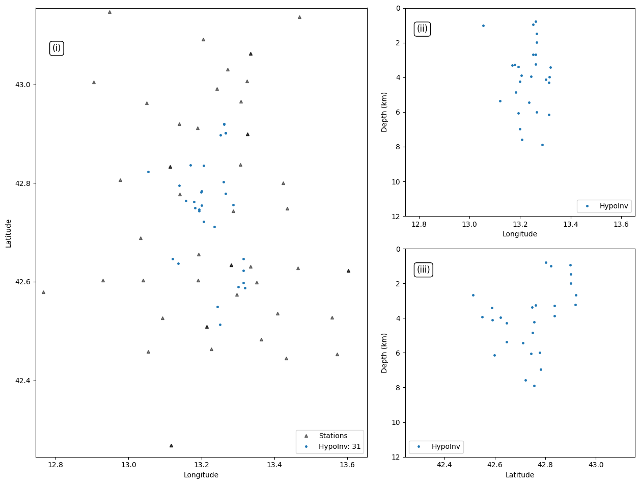
print(len(events_hpy))
31
Plot event locations:#
marker_size=5
hyp_label="HypoInv"
fig = plt.figure(figsize=plt.rcParams["figure.figsize"]*np.array([2,2]))
box = dict(boxstyle='round', facecolor='white', alpha=1)
text_loc = [0.05, 0.92]
grd = fig.add_gridspec(ncols=2, nrows=2, width_ratios=[1.5, 1], height_ratios=[1,1])
fig.add_subplot(grd[:, 0])
plt.plot(stations["longitude"], stations["latitude"], 'k^', markersize=marker_size, alpha=0.5, label="Stations")
plt.plot(events_hpy["LON"], events_hpy["LAT"], '.',markersize=marker_size, alpha=1.0, rasterized=True, label=f"{hyp_label}: {len(events_hpy)}")

plt.gca().set_aspect(111/82)
plt.xlim(np.array(config["xlim_degree"])+np.array([-0.03,0.03]))
plt.ylim(np.array(config["ylim_degree"])+np.array([-0.03,0.03]))
plt.ylabel("Latitude")
plt.xlabel("Longitude")
plt.gca().set_prop_cycle(None)
plt.plot(config["xlim_degree"][0]-10, config["ylim_degree"][0]-10, '.', markersize=10)
plt.legend(loc="lower right")
plt.text(text_loc[0], text_loc[1], '(i)', horizontalalignment='left', verticalalignment="top",
         transform=plt.gca().transAxes, fontsize="large", fontweight="normal", bbox=box)

fig.add_subplot(grd[0, 1])
plt.plot(events_hpy["LON"], events_hpy["DEPTH"], '.', markersize=marker_size, alpha=1.0, rasterized=True,label=f"{hyp_label}")

plt.xlim(np.array(config["xlim_degree"])+np.array([-0.03,0.03]))
plt.ylim(bottom=0, top=12)
plt.gca().invert_yaxis()
plt.xlabel("Longitude")
plt.ylabel("Depth (km)")
plt.gca().set_prop_cycle(None)
plt.plot(config["xlim_degree"][0]-10, 31, '.', markersize=10)
plt.legend(loc="lower right")
plt.text(text_loc[0], text_loc[1], '(ii)', horizontalalignment='left', verticalalignment="top",
         transform=plt.gca().transAxes, fontsize="large", fontweight="normal", bbox=box)


fig.add_subplot(grd[1, 1])
plt.plot(events_hpy["LAT"], events_hpy["DEPTH"], '.', markersize=marker_size, alpha=1.0, rasterized=True,label=f"{hyp_label}")

plt.xlim(np.array(config["ylim_degree"])+np.array([-0.03,0.03]))
plt.ylim(bottom=0, top=12)
plt.gca().invert_yaxis()
plt.xlabel("Latitude")
plt.ylabel("Depth (km)")
plt.gca().set_prop_cycle(None)
plt.plot(config["ylim_degree"][0]-10, 31, '.', markersize=10)
plt.legend(loc="lower left")
plt.tight_layout()
plt.text(text_loc[0], text_loc[1], '(iii)', horizontalalignment='left', verticalalignment="top",
         transform=plt.gca().transAxes, fontsize="large", fontweight="normal", bbox=box)

plt.show()
HypoDD#
Run with test data (10 min, ~30 events)
When running HypoDD, you may need to change the .inp files.
See HypoDD manual (https://github.com/fwaldhauser/HypoDD)
Write phase file from HypoInverese output#
import datetime
import math
import sys
import os

def format_convert(phaseinput,phaseoutput):

    g = open(phaseoutput, 'w')
    nn = 100000

    with open(phaseinput, "r") as f:
        for line in f:
            if (len(line) == 180):
                iok = 0
                RMS = float(line[48:52]) / 100
                gap = int(line[42:45])
                dep = float(line[31:36])/100
                EZ = float(line[89:93])/100
                EH = float(line[85:89])/100

                nn = nn + 1
                year = int(line[0:4])
                mon = int(line[4:6])
                day = int(line[6:8])
                hour = int(line[8:10])
                min = int(line[10:12])
                sec = int(line[12:16])/100

                if line[18] == ' ': #N
                    lat = (float(line[16:18]) + float(line[19:23]) / 6000)
                else:
                    lat = float(line[16:18]) + float(line[19:23])/6000 * (-1)

                if line[26] == 'E':
                    lon = (float(line[23:26]) + float(line[27:31]) / 6000)
                else:
                    lon = (float(line[23:26]) + float(line[27:31]) / 6000) * (-1)

                mag = float(line[123:126])/100
                g.write(
                    '# {:4d} {:2d} {:2d} {:2d} {:2d} {:5.2f}  {:7.4f} {:9.4f}   {:5.2f} {:5.2f} {:5.2f} {:5.2f} {:5.2f} {:9d} E\n'.format(
                        year, mon, day, hour, min, sec, lat, lon, dep, mag, EH, EZ, RMS, nn))
                iok = 1
            else:
                if (iok == 1 and len(line) == 121):
                    station = line[0:5]
                    net = line[5:7]
                    chn = line[9:11]
                    year1 = int(line[17:21])
                    mon1 = int(line[21:23])
                    day1 = int(line[23:25])
                    hour1 = int(line[25:27])
                    min1 = int(line[27:29])

                    if year1 == year and mon1 == mon and day1 == day and hour1 == hour and min1 == min:
                        sec_p =sec
                        if line[13:15] == ' P' or line[13:15] == 'IP':
                            P_residual = abs(int(line[34:38]) / 100)
                            sec_p = int(line[29:34]) / 100
                            ppick = sec_p-sec

                            g.write('{:<2s}{:<5s}    {:8.3f}   1.000   P {:<2s} \n'.format(net, station, ppick,chn))

                        if line[46:48] == ' S' or line[46:48] == 'ES':
                            S_residual = abs(int(line[50:54]) / 100)
                            sec_s = int(line[41:46]) / 100
                            spick = sec_s-sec

                            g.write('{:<2s}{:<5s}    {:8.3f}   1.000   S {:<2s} \n'.format(net, station, spick,chn))
    f.close()
    g.close()

%cd /app
input_file = './hypoInv/hypoOut.arc'
Path('./hypodd/results_hypodd').mkdir(parents=True, exist_ok=True)
output_file = './hypodd/results_hypodd/hypoDD.pha'
format_convert(input_file, output_file)
print('phase file:', output_file)
%cp stations_hypoDD.dat ./hypodd/results_hypodd/.
/app
phase file: ./hypodd/results_hypodd/hypoDD.pha
Convert phase file to time difference file (dt.ct)#
%cd /app/hypodd/results_hypodd
%pwd
!ph2dt ph2dt.inp
/app/hypodd/results_hypodd
starting ph2dt (v2.1b - 08/2012)...     Sun Apr 28 00:50:55 2024
reading data ...
 > stations =           92
 > events total =           31
 > events selected =           31
 > phases =          834
forming dtimes...
 > stations selected =           35
 > P-phase pairs total =         1012
 > S-phase pairs total =         1218
 > outliers =           65  (           2 %)
 > phases at stations not in station list =            0
 > phases at distances larger than MAXDIST =            0
 > P-phase pairs selected =          941  (          92 %)
 > S-phase pairs selected =         1145  (          94 %)
 > weakly linked events =           31  (         100 %)
 > linked event pairs =          138
 > average links per pair =           15
 > average offset (km) betw. linked events =    6.95590639
 > average offset (km) betw. strongly linked events =    6.96204662
 > maximum offset (km) betw. strongly linked events =    11.9371490

Done.  Sun Apr 28 00:50:55 2024
Output files: dt.ct; event.dat; event.sel; station.sel; ph2dt.log
ph2dt parameters were:
(minwght,maxdist,maxsep,maxngh,minlnk,minobs,maxobs)
 0.01  150.000   12.000  50   5   8  60
Run double-difference relocation#
!hypoDD hypoDD.inp
starting hypoDD (v2.1beta - 06/15/2016)...   Sun Apr 28 00:50:55 2024Input parameters: hypoDD.inp (hypoDD2.0 format)
INPUT FILES:
 cross dtime data:
 catalog dtime data: dt.ct
 events: event.sel
 stations: station.sel
OUTPUT FILES:
 initial locations: hypoDD.loc
 relocated events: hypoDD.reloc
 event pair residuals: hypoDD.res
 station residuals: hypoDD.sta
 source parameters: hypoDD.src
Use local layered 1D model.
Relocate cluster number    1
Relocate all events
Remove air quakes.
Reading data ...   Sun Apr 28 00:50:55 2024
# events =    31
# stations < maxdist =     35
# stations w/ neg. elevation (set to 0) =    0
# catalog P dtimes =     724
# catalog S dtimes =     886
# dtimes total =     1610
# events after dtime match =         29
# stations =     34
clustering ...
Clustered events:    29
Isolated events:     0
# clusters:    1
Cluster   1:    29 events

RELOCATION OF CLUSTER: 1     Sun Apr 28 00:50:55 2024----------------------
Initial trial sources =    29
1D ray tracing.

  IT   EV  CT    RMSCT   RMSST   DX   DY   DZ   DT   OS  AQ  CND
        %   %   ms     %    ms    m    m    m   ms    m
 1    100 100  490  -0.4     0    5    5   14    1    0   2    3
 2     93  95  478  -2.3     0    5    4   12    1    0   1    3
 3  1  90  86  460  -3.7  1402    5    4   11    1    2   0    3
 4  2  90  84  399 -13.3  1402    6    4   10    1    4   0    3
 5  3  90  84  399   0.1  1402    6    4   10    1    6   0    3
 6  4  90  84  398  -0.5  1402    6    4   10    1    8   0    3
 7  5  90  84  396  -0.5  1402    6    4    9    1   10   0    3
 8  6  90  69  323 -18.4  1402    6    4   10    1   12   0    3
 9  7  90  68  301  -6.7   814    5    4    9    1   14   0    3
10  8  90  68  297  -1.2   814    5    4    9    1   16   0    3
11  9  90  68  295  -0.8   644    5    3    9    1   18   0    3
12 10  90  68  292  -1.0   641    5    3    8    1   19   0    3
13 11  90  59  245 -15.9   757    5    4    8    1   21   0    3
14 12  90  58  237  -3.5   757    5    3    8    1   22   0    3
15 13  90  58  233  -1.4   757    5    3    7    1   23   0    3
16 14  90  58  232  -0.7   757    5    3    7    1   24   0    3
17 15  90  58  231  -0.5   757    5    3    7    1   25   0    3

writing out results ...
   Program hypoDD finished. Sun Apr 28 00:50:55 2024
Read HypoDD output#
events_hypodd = pd.read_csv('./hypoDD.reloc',header=None, sep="\s+",names=['ID', 'LAT', 'LON', 'DEPTH', 'X', 'Y', 'Z', 'EX', 'EY', 'EZ', 'YR', 'MO', 'DY', 'HR', 'MI', 'SC', 'MAG', 'NCCP', 'NCCS', 'NCTP', 'NCTS', 'RCC', 'RCT', 'CID'])
events_hypodd
| ID | LAT | LON | DEPTH | X | Y | Z | EX | EY | EZ | ... | MI | SC | MAG | NCCP | NCCS | NCTP | NCTS | RCC | RCT | CID | |
|---|---|---|---|---|---|---|---|---|---|---|---|---|---|---|---|---|---|---|---|---|---|
| 0 | 100001 | 42.897148 | 13.251325 | 0.998 | 1659.9 | 16185.4 | -2882.9 | 423.3 | 463.1 | 518.6 | ... | 0 | 13.09 | 0.0 | 0 | 0 | 15 | 23 | -9.0 | 0.155 | 1 |
| 1 | 100003 | 42.748539 | 13.184111 | 4.796 | -3841.1 | -323.2 | 914.7 | 668.6 | 424.0 | 371.6 | ... | 0 | 55.47 | 0.0 | 0 | 0 | 44 | 45 | -9.0 | 0.302 | 1 |
| 2 | 100004 | 42.836003 | 13.172145 | 3.487 | -4817.4 | 9392.9 | -393.7 | 1138.7 | 976.9 | 1431.5 | ... | 1 | 43.87 | 0.0 | 0 | 0 | 9 | 12 | -9.0 | 0.554 | 1 |
| 3 | 100005 | 42.711308 | 13.234213 | 5.847 | 260.9 | -4459.2 | 1965.5 | 508.5 | 704.8 | 922.3 | ... | 2 | 8.92 | 0.0 | 0 | 0 | 48 | 47 | -9.0 | 0.643 | 1 |
| 4 | 100006 | 42.761275 | 13.179859 | 3.032 | -4188.7 | 1091.6 | -849.1 | 211.5 | 341.2 | 746.9 | ... | 2 | 41.51 | 0.0 | 0 | 0 | 69 | 76 | -9.0 | 0.296 | 1 |
| 5 | 100007 | 42.901440 | 13.266522 | 1.617 | 2902.4 | 16662.3 | -2264.5 | 335.5 | 291.1 | 592.0 | ... | 2 | 50.72 | 0.0 | 0 | 0 | 35 | 41 | -9.0 | 0.225 | 1 |
| 6 | 100008 | 42.721415 | 13.207220 | 7.610 | -1949.5 | -3336.3 | 3728.5 | 267.2 | 413.0 | 583.5 | ... | 3 | 32.59 | 0.0 | 0 | 0 | 57 | 88 | -9.0 | 0.276 | 1 |
| 7 | 100009 | 42.754818 | 13.198613 | 4.533 | -2653.6 | 374.3 | 652.3 | 556.9 | 613.5 | 839.6 | ... | 3 | 47.86 | 0.0 | 0 | 0 | 51 | 64 | -9.0 | 0.305 | 1 |
| 8 | 100010 | 42.901575 | 13.266191 | 1.894 | 2875.3 | 16677.2 | -1986.6 | 162.6 | 273.8 | 624.9 | ... | 4 | 1.42 | 0.0 | 0 | 0 | 36 | 40 | -9.0 | 0.167 | 1 |
| 9 | 100011 | 42.747160 | 13.193774 | 3.438 | -3049.9 | -476.4 | -443.4 | 221.1 | 264.8 | 581.1 | ... | 4 | 22.48 | 0.0 | 0 | 0 | 67 | 78 | -9.0 | 0.332 | 1 |
| 10 | 100012 | 42.586816 | 13.320344 | 3.425 | 7321.9 | -18288.7 | -455.6 | 473.9 | 459.2 | 588.8 | ... | 4 | 28.80 | 0.0 | 0 | 0 | 32 | 26 | -9.0 | 0.210 | 1 |
| 11 | 100013 | 42.597795 | 13.314291 | 6.218 | 6825.1 | -17069.1 | 2337.0 | 678.6 | 428.3 | 655.0 | ... | 4 | 37.25 | 0.0 | 0 | 0 | 16 | 20 | -9.0 | 0.176 | 1 |
| 12 | 100015 | 42.513460 | 13.250963 | 2.647 | 1635.3 | -26437.6 | -1233.9 | 338.3 | 477.3 | 654.8 | ... | 5 | 18.14 | 0.0 | 0 | 0 | 11 | 11 | -9.0 | 0.086 | 1 |
| 13 | 100016 | 42.802157 | 13.262620 | 10.812 | 2585.4 | 5633.1 | 6931.4 | 773.8 | 369.5 | 704.8 | ... | 5 | 31.98 | 0.0 | 0 | 0 | 15 | 20 | -9.0 | 0.525 | 1 |
| 14 | 100017 | 42.764795 | 13.156978 | 0.153 | -6061.6 | 1482.6 | -3727.8 | 460.1 | 367.6 | 592.5 | ... | 5 | 48.61 | 0.0 | 0 | 0 | 36 | 42 | -9.0 | 0.319 | 1 |
| 15 | 100018 | 42.622375 | 13.314778 | 3.953 | 6863.6 | -14338.5 | 72.0 | 371.9 | 228.0 | 276.7 | ... | 6 | 8.11 | 0.0 | 0 | 0 | 29 | 27 | -9.0 | 0.155 | 1 |
| 16 | 100021 | 42.836149 | 13.202519 | 3.647 | -2332.4 | 9409.2 | -234.4 | 1134.7 | 957.6 | 1588.4 | ... | 6 | 35.34 | 0.0 | 0 | 0 | 5 | 10 | -9.0 | 0.648 | 1 |
| 17 | 100022 | 42.918144 | 13.262372 | 3.376 | 2562.7 | 18517.8 | -505.4 | 198.9 | 385.5 | 581.8 | ... | 6 | 53.51 | 0.0 | 0 | 0 | 28 | 30 | -9.0 | 0.218 | 1 |
| 18 | 100023 | 42.777946 | 13.265730 | 6.328 | 2840.5 | 2943.5 | 2448.3 | 699.9 | 345.6 | 962.7 | ... | 7 | 17.84 | 0.0 | 0 | 0 | 23 | 33 | -9.0 | 0.545 | 1 |
| 19 | 100024 | 42.646944 | 13.315711 | 4.291 | 6938.8 | -11609.2 | 409.8 | 480.7 | 289.9 | 310.1 | ... | 7 | 26.49 | 0.0 | 0 | 0 | 29 | 30 | -9.0 | 0.206 | 1 |
| 20 | 100026 | 42.758439 | 13.283857 | 7.404 | 4324.9 | 776.6 | 3523.4 | 1390.2 | 931.3 | 1160.6 | ... | 8 | 10.19 | 0.0 | 0 | 0 | 25 | 28 | -9.0 | 0.391 | 1 |
| 21 | 100027 | 42.590499 | 13.301509 | 4.093 | 5777.7 | -17879.6 | 211.6 | 483.0 | 334.3 | 491.9 | ... | 8 | 25.08 | 0.0 | 0 | 0 | 28 | 32 | -9.0 | 0.160 | 1 |
| 22 | 100028 | 42.549207 | 13.243958 | 3.992 | 1060.3 | -22466.7 | 110.8 | 387.3 | 429.4 | 636.7 | ... | 8 | 31.90 | 0.0 | 0 | 0 | 23 | 24 | -9.0 | 0.125 | 1 |
| 23 | 100029 | 42.782186 | 13.198467 | 6.883 | -2665.0 | 3414.5 | 3001.5 | 542.5 | 567.1 | 655.8 | ... | 8 | 42.18 | 0.0 | 0 | 0 | 23 | 40 | -9.0 | 0.415 | 1 |
| 24 | 100030 | 42.920585 | 13.261839 | 2.727 | 2519.1 | 18789.0 | -1154.0 | 247.2 | 206.3 | 448.6 | ... | 8 | 54.90 | 0.0 | 0 | 0 | 24 | 28 | -9.0 | 0.136 | 1 |
| 25 | 100031 | 42.743754 | 13.192710 | 5.961 | -3137.1 | -854.8 | 2079.9 | 278.3 | 479.8 | 519.5 | ... | 9 | 23.21 | 0.0 | 0 | 0 | 74 | 93 | -9.0 | 0.350 | 1 |
26 rows × 24 columns
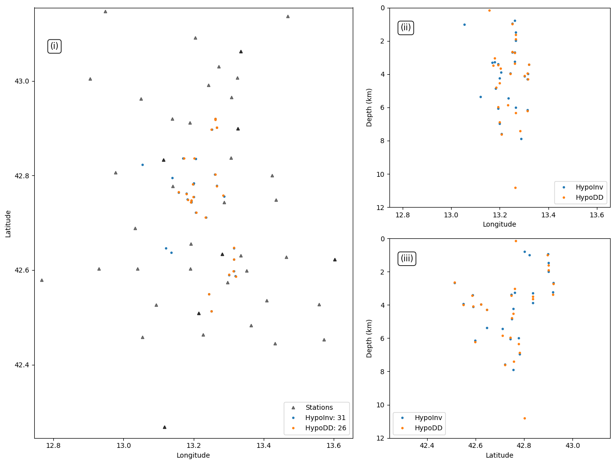
Plot event locations#
marker_size=5
hyp_label="HypoInv"
hypodd_label='HypoDD'
fig = plt.figure(figsize=plt.rcParams["figure.figsize"]*np.array([2,2]))
box = dict(boxstyle='round', facecolor='white', alpha=1)
text_loc = [0.05, 0.92]
grd = fig.add_gridspec(ncols=2, nrows=2, width_ratios=[1.5, 1], height_ratios=[1,1])
fig.add_subplot(grd[:, 0])
plt.plot(stations["longitude"], stations["latitude"], 'k^', markersize=marker_size, alpha=0.5, label="Stations")
plt.plot(events_hpy["LON"], events_hpy["LAT"], '.',markersize=marker_size, alpha=1.0, rasterized=True, label=f"{hyp_label}: {len(events_hpy)}")
plt.plot(events_hypodd["LON"], events_hypodd["LAT"], '.',markersize=marker_size, alpha=1.0, rasterized=True, label=f"{hypodd_label}: {len(events_hypodd)}")


plt.gca().set_aspect(111/82)
plt.xlim(np.array(config["xlim_degree"])+np.array([-0.03,0.03]))
plt.ylim(np.array(config["ylim_degree"])+np.array([-0.03,0.03]))
plt.ylabel("Latitude")
plt.xlabel("Longitude")
plt.gca().set_prop_cycle(None)
plt.plot(config["xlim_degree"][0]-10, config["ylim_degree"][0]-10, '.', markersize=10)
plt.legend(loc="lower right")
plt.text(text_loc[0], text_loc[1], '(i)', horizontalalignment='left', verticalalignment="top",
         transform=plt.gca().transAxes, fontsize="large", fontweight="normal", bbox=box)

fig.add_subplot(grd[0, 1])
plt.plot(events_hpy["LON"], events_hpy["DEPTH"], '.', markersize=marker_size, alpha=1.0, rasterized=True,label=f"{hyp_label}")
plt.plot(events_hypodd["LON"], events_hypodd["DEPTH"], '.', markersize=marker_size, alpha=1.0, rasterized=True,label=f"{hypodd_label}")

plt.xlim(np.array(config["xlim_degree"])+np.array([-0.03,0.03]))
plt.ylim(bottom=0, top=12)
plt.gca().invert_yaxis()
plt.xlabel("Longitude")
plt.ylabel("Depth (km)")
plt.gca().set_prop_cycle(None)
plt.plot(config["xlim_degree"][0]-10, 31, '.', markersize=10)
plt.legend(loc="lower right")
plt.text(text_loc[0], text_loc[1], '(ii)', horizontalalignment='left', verticalalignment="top",
         transform=plt.gca().transAxes, fontsize="large", fontweight="normal", bbox=box)


fig.add_subplot(grd[1, 1])
plt.plot(events_hpy["LAT"], events_hpy["DEPTH"], '.', markersize=marker_size, alpha=1.0, rasterized=True,label=f"{hyp_label}")
plt.plot(events_hypodd["LAT"], events_hypodd["DEPTH"], '.', markersize=marker_size, alpha=1.0, rasterized=True,label=f"{hypodd_label}")

plt.xlim(np.array(config["ylim_degree"])+np.array([-0.03,0.03]))
plt.ylim(bottom=0, top=12)
plt.gca().invert_yaxis()
plt.xlabel("Latitude")
plt.ylabel("Depth (km)")
plt.gca().set_prop_cycle(None)
plt.plot(config["ylim_degree"][0]-10, 31, '.', markersize=10)
plt.legend(loc="lower left")
plt.tight_layout()
plt.text(text_loc[0], text_loc[1], '(iii)', horizontalalignment='left', verticalalignment="top",
         transform=plt.gca().transAxes, fontsize="large", fontweight="normal", bbox=box)

plt.show()
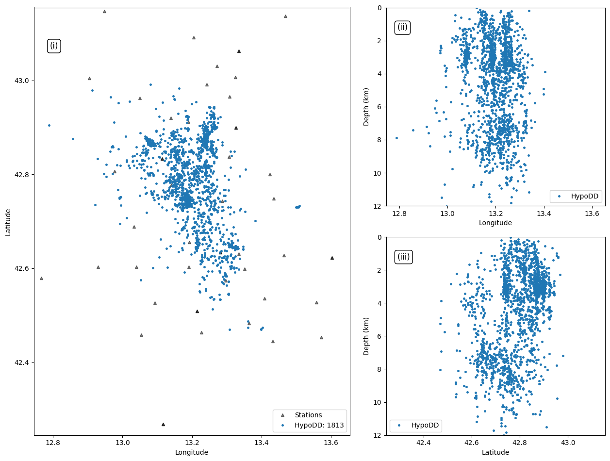
HypoDD (example)#
We provide an example of one day (2016/10/18) data in the Amatrice, Italy sequence to test run HypoDD. The input phase file is generated using the same workflow introduced in this tutorial notebook.
Convert phase file to time difference file (dt.ct)#
%cd /app/hypodd/hypodd_example
%pwd
!ph2dt ph2dt.inp
/app/hypodd/hypodd_example
starting ph2dt (v2.1b - 08/2012)...     Sun Apr 28 00:50:56 2024
reading data ...
 > stations =           67
 > events total =         2635
 > events selected =         2635
 > phases =        82478
forming dtimes...
 > stations selected =           52
 > P-phase pairs total =       933760
 > S-phase pairs total =      1116260
 > outliers =       112326  (           5 %)
 > phases at stations not in station list =       707399
 > phases at distances larger than MAXDIST =            0
 > P-phase pairs selected =       382488  (          40 %)
 > S-phase pairs selected =       484074  (          43 %)
 > weakly linked events =          161  (           6 %)
 > linked event pairs =        54670
 > average links per pair =           15
 > average offset (km) betw. linked events =    2.41818690
 > average offset (km) betw. strongly linked events =    2.89636850
 > maximum offset (km) betw. strongly linked events =    11.9986162

Done.  Sun Apr 28 00:50:59 2024
Output files: dt.ct; event.dat; event.sel; station.sel; ph2dt.log
ph2dt parameters were:
(minwght,maxdist,maxsep,maxngh,minlnk,minobs,maxobs)
 0.01  150.000   12.000  50   5   8  60
Run double-difference relocation#
!hypoDD hypoDD.inp
starting hypoDD (v2.1beta - 06/15/2016)...   Sun Apr 28 00:50:59 2024Input parameters: hypoDD.inp (hypoDD2.0 format)
INPUT FILES:
 cross dtime data:
 catalog dtime data: dt.ct
 events: event.sel
 stations: station.sel
OUTPUT FILES:
 initial locations: hypoDD.loc
 relocated events: hypoDD.reloc
 event pair residuals: hypoDD.res
 station residuals: hypoDD.sta
 source parameters: hypoDD.src
Use local layered 1D model.
Relocate cluster number    1
Relocate all events
Remove air quakes.
Reading data ...   Sun Apr 28 00:50:59 2024
# events =  2635
# stations < maxdist =     52
# stations w/ neg. elevation (set to 0) =    0
# catalog P dtimes =  380059
# catalog S dtimes =  481342
# dtimes total =   861401
# events after dtime match =       2263
# stations =     47
clustering ...
Clustered events:  1972
Isolated events:   291
# clusters:    4
Cluster   1:  1965 events
Cluster   2:     3 events
Cluster   3:     2 events
Cluster   4:     2 events

RELOCATION OF CLUSTER: 1     Sun Apr 28 00:51:00 2024----------------------
Reading data ...   Sun Apr 28 00:51:00 2024�
# events =  1965
# stations < maxdist =     52
# stations w/ neg. elevation (set to 0) =    0
# catalog P dtimes =  360824
# catalog S dtimes =  457339
# dtimes total =   818163
# events after dtime match =       1965
# stations =     47
Initial trial sources =  1965
1D ray tracing.

  IT   EV  CT    RMSCT   RMSST   DX   DY   DZ   DT   OS  AQ  CND
        %   %   ms     %    ms    m    m    m   ms    m
 1    100 100  244 -18.7     0  433  377  901   79    0  48   62
 2  1  98  98  240  -1.7   512  424  364  832   76  115   0   60
 3     97  97  182 -24.2   512  144  144  328   31  115  18   71
 4     96  96  180  -1.3   512  140  142  308   31  115   1   69
 5  2  96  96  179  -0.3   517  140  142  308   31   43   0   69
 6     96  96  166  -7.1   517   83   80  198   17   43  14   67
 7  3  96  95  165  -0.7   411   82   78  188   17   48   0   67
 8     96  95  159  -3.6   411   59   54  151   12   48   7   65
 9  4  95  94  159  -0.5   407   59   54  145   12   55   0   65
10     95  94  155  -2.2   407   42   42  117    9   55   5   64
11  5  95  94  155  -0.3   415   42   41  115    9   67   0   63
12     95  92  135 -12.5   415   57   58  135   11   67   5   87
13  6  95  92  134  -1.2   408   58   59  133   11   71   0   87
14     95  92  128  -4.0   408   44   47  104    8   71   5   84
15  7  94  91  128  -0.5   406   44   46  100    8   82   0   84
16     94  91  125  -2.4   406   35   34   87    7   82   4   85
17  8  94  91  124  -0.3   406   35   34   84    7   88   0   85
18     94  91  122  -1.5   406   27   25   73    5   88   3   80
19  9  94  90  122  -0.3   413   27   26   73    5   94   0   80
20     94  90  121  -1.0   413   21   22   62    4   94   3   80
21 10  93  90  121  -0.2   421   21   22   62    4  102   0   80
22     93  88  102 -15.2   421   32   36   78    7  102   2   81
23 11  93  87  100  -1.9   450   33   38   79    7  106   0   81
24     93  87   96  -4.2   450   24   26   68    5  106   4   82
25 12  93  87   96  -0.5   355   25   26   68    5  111   0   81
26     93  86   93  -2.3   355   18   19   65    4  111   4   80
27 13  93  86   93  -0.4   360   18   19   63    4  119   0   80
28     92  86   92  -1.4   360   14   15   50    3  119   3   80
29 14  92  86   91  -0.3   367   14   15   49    3  129   0   80
30 15  92  85   91  -0.9   366   12   13   41    3  131   0   78

writing out results ...
   Program hypoDD finished. Sun Apr 28 00:52:01 2024
Read HypoDD output#
events_hypodd = pd.read_csv('./hypoDD.reloc',header=None, sep="\s+",names=['ID', 'LAT', 'LON', 'DEPTH', 'X', 'Y', 'Z', 'EX', 'EY', 'EZ', 'YR', 'MO', 'DY', 'HR', 'MI', 'SC', 'MAG', 'NCCP', 'NCCS', 'NCTP', 'NCTS', 'RCC', 'RCT', 'CID'])
events_hypodd
| ID | LAT | LON | DEPTH | X | Y | Z | EX | EY | EZ | ... | MI | SC | MAG | NCCP | NCCS | NCTP | NCTS | RCC | RCT | CID | |
|---|---|---|---|---|---|---|---|---|---|---|---|---|---|---|---|---|---|---|---|---|---|
| 0 | 113825 | 42.900224 | 13.256211 | 3.249 | 4497.0 | 12620.9 | -1405.3 | 143.2 | 193.8 | 333.9 | ... | 0 | 12.80 | 0.0 | 0 | 0 | 368 | 417 | -9.0 | 0.168 | 1 |
| 1 | 113827 | 42.742236 | 13.194716 | 5.578 | -530.7 | -4929.7 | 923.8 | 159.1 | 174.6 | 172.3 | ... | 0 | 55.20 | 0.0 | 0 | 0 | 393 | 464 | -9.0 | 0.138 | 1 |
| 2 | 113829 | 42.836812 | 13.162251 | 5.476 | -3185.7 | 5576.6 | 821.7 | 130.2 | 104.5 | 167.8 | ... | 1 | 43.52 | 0.0 | 0 | 0 | 589 | 733 | -9.0 | 0.132 | 1 |
| 3 | 113830 | 42.710832 | 13.228359 | 5.398 | 2223.5 | -8418.4 | 744.1 | 222.3 | 183.7 | 345.1 | ... | 2 | 9.29 | 0.0 | 0 | 0 | 231 | 48 | -9.0 | 0.185 | 1 |
| 4 | 113831 | 42.756763 | 13.179973 | 2.664 | -1737.3 | -3316.0 | -1990.1 | 150.9 | 194.3 | 266.2 | ... | 2 | 41.27 | 0.0 | 0 | 0 | 482 | 556 | -9.0 | 0.120 | 1 |
| ... | ... | ... | ... | ... | ... | ... | ... | ... | ... | ... | ... | ... | ... | ... | ... | ... | ... | ... | ... | ... | ... |
| 1808 | 116488 | 42.800183 | 13.190090 | 5.220 | -909.0 | 1507.5 | 565.6 | 126.7 | 131.7 | 225.4 | ... | 55 | 34.78 | 0.0 | 0 | 0 | 110 | 239 | -9.0 | 0.119 | 1 |
| 1809 | 116489 | 42.661751 | 13.218293 | 7.283 | 1400.0 | -13870.7 | 2628.9 | 116.7 | 143.2 | 242.2 | ... | 56 | 6.20 | 0.0 | 0 | 0 | 314 | 426 | -9.0 | 0.108 | 1 |
| 1810 | 116492 | 42.817647 | 13.181880 | 2.591 | -1580.5 | 3447.6 | -2063.3 | 135.1 | 106.2 | 202.4 | ... | 57 | 33.16 | 0.0 | 0 | 0 | 690 | 775 | -9.0 | 0.151 | 1 |
| 1811 | 116494 | 42.869812 | 13.176278 | 1.597 | -2037.9 | 9242.5 | -3057.7 | 149.5 | 122.2 | 187.0 | ... | 59 | 12.40 | 0.0 | 0 | 0 | 381 | 536 | -9.0 | 0.161 | 1 |
| 1812 | 116495 | 42.840857 | 13.154974 | 6.886 | -3780.7 | 6025.9 | 2231.8 | 180.8 | 164.4 | 199.3 | ... | 59 | 31.44 | 0.0 | 0 | 0 | 118 | 301 | -9.0 | 0.161 | 1 |
1813 rows × 24 columns
Plot event locations of the 1-day example#
marker_size=5
hyp_label="HypoInv"
hypodd_label='HypoDD'
fig = plt.figure(figsize=plt.rcParams["figure.figsize"]*np.array([2,2]))
box = dict(boxstyle='round', facecolor='white', alpha=1)
text_loc = [0.05, 0.92]
grd = fig.add_gridspec(ncols=2, nrows=2, width_ratios=[1.5, 1], height_ratios=[1,1])
fig.add_subplot(grd[:, 0])
plt.plot(stations["longitude"], stations["latitude"], 'k^', markersize=marker_size, alpha=0.5, label="Stations")
# plt.plot(events_hpy["LON"], events_hpy["LAT"], '.',markersize=marker_size, alpha=1.0, rasterized=True, label=f"{hyp_label}: {len(events_hpy)}")
plt.plot(events_hypodd["LON"], events_hypodd["LAT"], '.',markersize=marker_size, alpha=1.0, rasterized=True, label=f"{hypodd_label}: {len(events_hypodd)}")


plt.gca().set_aspect(111/82)
plt.xlim(np.array(config["xlim_degree"])+np.array([-0.03,0.03]))
plt.ylim(np.array(config["ylim_degree"])+np.array([-0.03,0.03]))
plt.ylabel("Latitude")
plt.xlabel("Longitude")
plt.gca().set_prop_cycle(None)
plt.plot(config["xlim_degree"][0]-10, config["ylim_degree"][0]-10, '.', markersize=10)
plt.legend(loc="lower right")
plt.text(text_loc[0], text_loc[1], '(i)', horizontalalignment='left', verticalalignment="top",
         transform=plt.gca().transAxes, fontsize="large", fontweight="normal", bbox=box)

fig.add_subplot(grd[0, 1])
# plt.plot(events_hpy["LON"], events_hpy["DEPTH"], '.', markersize=marker_size, alpha=1.0, rasterized=True,label=f"{hyp_label}")
plt.plot(events_hypodd["LON"], events_hypodd["DEPTH"], '.', markersize=marker_size, alpha=1.0, rasterized=True,label=f"{hypodd_label}")

plt.xlim(np.array(config["xlim_degree"])+np.array([-0.03,0.03]))
plt.ylim(bottom=0, top=12)
plt.gca().invert_yaxis()
plt.xlabel("Longitude")
plt.ylabel("Depth (km)")
plt.gca().set_prop_cycle(None)
plt.plot(config["xlim_degree"][0]-10, 31, '.', markersize=10)
plt.legend(loc="lower right")
plt.text(text_loc[0], text_loc[1], '(ii)', horizontalalignment='left', verticalalignment="top",
         transform=plt.gca().transAxes, fontsize="large", fontweight="normal", bbox=box)


fig.add_subplot(grd[1, 1])
# plt.plot(events_hpy["LAT"], events_hpy["DEPTH"], '.', markersize=marker_size, alpha=1.0, rasterized=True,label=f"{hyp_label}")
plt.plot(events_hypodd["LAT"], events_hypodd["DEPTH"], '.', markersize=marker_size, alpha=1.0, rasterized=True,label=f"{hypodd_label}")

plt.xlim(np.array(config["ylim_degree"])+np.array([-0.03,0.03]))
plt.ylim(bottom=0, top=12)
plt.gca().invert_yaxis()
plt.xlabel("Latitude")
plt.ylabel("Depth (km)")
plt.gca().set_prop_cycle(None)
plt.plot(config["ylim_degree"][0]-10, 31, '.', markersize=10)
plt.legend(loc="lower left")
plt.tight_layout()
plt.text(text_loc[0], text_loc[1], '(iii)', horizontalalignment='left', verticalalignment="top",
         transform=plt.gca().transAxes, fontsize="large", fontweight="normal", bbox=box)

plt.show()